Survival Analysis Exercises

In this document we will conduct survival analysis on a data set relating employee turnover to several variables that were measured at the time an employee was hired.

Exercise 1 - Load, explore, and structure the survival data

library(dplyr)

Attaching package: 'dplyr'

The following objects are masked from 'package:stats':

    filter, lag

The following objects are masked from 'package:base':

    intersect, setdiff, setequal, union

library(survival)
library(survminer)

Loading required package: ggplot2

Loading required package: ggpubr

Attaching package: 'survminer'

The following object is masked from 'package:survival':

    myeloma

library(lubridate)

Attaching package: 'lubridate'

The following objects are masked from 'package:base':

    date, intersect, setdiff, union

# Load the survival analysis data file from the url provided
url <- "https://rstudio-conf-2022.github.io/people-analytics-rstats/data/survival_analysis_data.csv"
surv_data <- read.csv(url)

# view the first few rows in the data set to acquaint yourself with the data
head(surv_data)

     EID REFERRAL NUMBER_JOBS PROG_EXER_RATE INTPER_RATE PRIOR_EXP HIRE_REC
1 453921       No           2           Pass           6       Yes        2
2 732470       No          3+           Pass          10        No        2
3 169619       No          3+       Concerns          10        No        1
4 953421       No         0-1       Concerns           6        No        2
5 363973       No           2           Pass          10       Yes        3
6 779914       No         0-1           Pass           7        No        2
   HIRE_DATE TURNOVER_DATE TURNOVER
1 2017-02-01          <NA>       No
2 2016-02-01    2017-12-01      Yes
3 2016-02-01          <NA>       No
4 2017-02-01    2017-07-01      Yes
5 2016-02-01          <NA>       No
6 2017-01-01    2021-01-01      Yes

# convert columns ending in 'DATE' to date format
surv_data <- surv_data |> 
  dplyr::mutate(across(ends_with("DATE"), as.Date))

# Create a censor indicator variable that is 1 if the employee has left and 0 otherwise
surv_data <- 
  surv_data |> 
  dplyr::mutate(
    CENSOR = dplyr::case_when(
      TURNOVER == "Yes" ~ 1,
      TRUE ~ 0
    )
  )

# Replace missing TURNOVER_DATE values with "2022-07-01" -- think about what missing TURNOVER_DATES mean
surv_data <- 
  surv_data |>
  dplyr::mutate(
    TURNOVER_DATE = dplyr::case_when(
      is.na(TURNOVER_DATE) ~ as.Date("2022-07-01"),
      TRUE ~ TURNOVER_DATE
    )
  )

# Use the lubridate::interval() function to create the EVENT_TIME variable 
# Hint: Use  %/% months(1) to transform the time difference into months 
surv_data <- 
  surv_data |>
  dplyr::mutate(
    EVENT_TIME = lubridate::interval(HIRE_DATE, TURNOVER_DATE) %/% months(1)
  )

# Calculate some descriptive statistics for EVENT_TIME using the full sample, then group the data by CENSOR to see how the descriptives
# change. 
mean(surv_data$EVENT_TIME)

[1] 43.20513

median(surv_data$EVENT_TIME)

[1] 47

surv_data |>
  dplyr::group_by(
    CENSOR
  ) |>
  dplyr::summarise(
    MEAN_EVENT_TIME = mean(EVENT_TIME),
    MEDIAN_EVENT_TIME = median(EVENT_TIME),
    SD_EVENT_TIME = sd(EVENT_TIME)
  )

# A tibble: 2 × 4
  CENSOR MEAN_EVENT_TIME MEDIAN_EVENT_TIME SD_EVENT_TIME
   <dbl>           <dbl>             <dbl>         <dbl>
1      0            69.9                66          6.54
2      1            28.0                27         17.6 

Exercise 2 - Create a survival object and estimate survival functions using Kaplan Meier estimates

# Create a survival object using survival::Surv().
# Remember it requires two arguments EVENT_TIME and CENSOR
surv_object <- survival::Surv(
  event = surv_data$CENSOR,
  time = surv_data$EVENT_TIME
)

# Use survival::survfit() to estimate survival probabilities using the Kaplan Meier estimator for the entire sample
# Save the survfit output into an object called km_all

# How many months after hiring would you expect 50% of the sample to remain at the firm? (e.g. the median survival time)
# How many months after hiring would you expect 75% of the sample to remain at the firm?

km_all <- survival::survfit(surv_object ~ 1, data = surv_data)
summary(km_all)

Call: survfit(formula = surv_object ~ 1, data = surv_data)

 time n.risk n.event survival std.err lower 95% CI upper 95% CI
    1   8000     182    0.977 0.00167        0.974        0.981
    2   7818     181    0.955 0.00233        0.950        0.959
    3   7637     187    0.931 0.00283        0.926        0.937
    4   7450     135    0.914 0.00313        0.908        0.921
    5   7315     128    0.898 0.00338        0.892        0.905
    6   7187     110    0.885 0.00357        0.878        0.892
    7   7077      87    0.874 0.00371        0.867        0.881
    8   6990      68    0.865 0.00382        0.858        0.873
    9   6922      41    0.860 0.00388        0.853        0.868
   10   6881      58    0.853 0.00396        0.845        0.861
   11   6823      36    0.848 0.00401        0.841        0.856
   12   6787      35    0.844 0.00406        0.836        0.852
   13   6752      27    0.841 0.00409        0.833        0.849
   14   6725      29    0.837 0.00413        0.829        0.845
   15   6696      38    0.832 0.00418        0.824        0.840
   16   6658      41    0.827 0.00423        0.819        0.835
   17   6617      36    0.823 0.00427        0.814        0.831
   18   6581      46    0.817 0.00432        0.808        0.825
   19   6535      57    0.810 0.00439        0.801        0.818
   20   6478      69    0.801 0.00446        0.792        0.810
   21   6409      93    0.789 0.00456        0.781        0.798
   22   6316     117    0.775 0.00467        0.766        0.784
   23   6199     134    0.758 0.00479        0.749        0.768
   24   6065     124    0.743 0.00489        0.733        0.752
   25   5941     163    0.722 0.00501        0.713        0.732
   26   5778     218    0.695 0.00515        0.685        0.705
   27   5560     197    0.670 0.00526        0.660        0.681
   28   5363     199    0.645 0.00535        0.635        0.656
   29   5164     178    0.623 0.00542        0.613        0.634
   30   4986     160    0.603 0.00547        0.593        0.614
   31   4826     117    0.589 0.00550        0.578        0.600
   32   4709      94    0.577 0.00552        0.566        0.588
   33   4615      76    0.567 0.00554        0.557        0.578
   34   4539      51    0.561 0.00555        0.550        0.572
   35   4488      32    0.557 0.00555        0.546        0.568
   36   4456      15    0.555 0.00556        0.544        0.566
   37   4441      12    0.554 0.00556        0.543        0.565
   38   4429      16    0.552 0.00556        0.541        0.563
   39   4413      15    0.550 0.00556        0.539        0.561
   40   4398      26    0.547 0.00557        0.536        0.558
   41   4372      47    0.541 0.00557        0.530        0.552
   42   4325      55    0.534 0.00558        0.523        0.545
   43   4270      59    0.526 0.00558        0.516        0.537
   44   4211      59    0.519 0.00559        0.508        0.530
   45   4152      85    0.508 0.00559        0.498        0.519
   46   4067      64    0.500 0.00559        0.490        0.511
   47   4003      83    0.490 0.00559        0.479        0.501
   48   3920     100    0.478 0.00558        0.467        0.489
   49   3820     122    0.462 0.00557        0.451        0.473
   50   3698      97    0.450 0.00556        0.439        0.461
   51   3601      90    0.439 0.00555        0.428        0.450
   52   3511      91    0.428 0.00553        0.417        0.438
   53   3420      88    0.417 0.00551        0.406        0.427
   54   3332      88    0.406 0.00549        0.395        0.416
   55   3244      68    0.397 0.00547        0.386        0.408
   56   3152      57    0.390 0.00545        0.379        0.401
   57   3088      41    0.385 0.00544        0.374        0.395
   58   3040      39    0.380 0.00543        0.369        0.390
   59   2951      39    0.375 0.00542        0.364        0.385
   60   2868      18    0.372 0.00541        0.362        0.383
   61   2813      11    0.371 0.00541        0.360        0.382
   62   2726       2    0.371 0.00541        0.360        0.381
   63   2645       3    0.370 0.00540        0.360        0.381
   64   2496       3    0.370 0.00540        0.359        0.380
   65   2353       1    0.370 0.00540        0.359        0.380
   67   1502       2    0.369 0.00541        0.359        0.380
   68   1485       9    0.367 0.00543        0.356        0.378
   69   1461       9    0.365 0.00545        0.354        0.375
   70   1445      10    0.362 0.00547        0.352        0.373
   71   1403      13    0.359 0.00549        0.348        0.370
   72   1348       9    0.356 0.00551        0.346        0.367

# Look at the structure of km_all using str()
str(km_all)

List of 16
 $ n        : int 8000
 $ time     : num [1:78] 1 2 3 4 5 6 7 8 9 10 ...
 $ n.risk   : num [1:78] 8000 7818 7637 7450 7315 ...
 $ n.event  : num [1:78] 182 181 187 135 128 110 87 68 41 58 ...
 $ n.censor : num [1:78] 0 0 0 0 0 0 0 0 0 0 ...
 $ surv     : num [1:78] 0.977 0.955 0.931 0.914 0.898 ...
 $ std.err  : num [1:78] 0.00171 0.00244 0.00304 0.00342 0.00376 ...
 $ cumhaz   : num [1:78] 0.0227 0.0459 0.0704 0.0885 0.106 ...
 $ std.chaz : num [1:78] 0.00169 0.00241 0.003 0.00338 0.00372 ...
 $ type     : chr "right"
 $ logse    : logi TRUE
 $ conf.int : num 0.95
 $ conf.type: chr "log"
 $ lower    : num [1:78] 0.974 0.95 0.926 0.908 0.892 ...
 $ upper    : num [1:78] 0.981 0.959 0.937 0.921 0.905 ...
 $ call     : language survfit(formula = surv_object ~ 1, data = surv_data)
 - attr(*, "class")= chr "survfit"

# Using km_all, create a new data frame called km_calc which contains the following variables from km_all:
# time, n.risk, n.censor, n.event, and surv 

km_calc <- 
  tibble::tibble(
    time = km_all$time,
    n.risk = km_all$n.risk,
    n.censor = km_all$n.censor,
    n.event = km_all$n.event,
    survival = km_all$surv
  )

# Using km_calc, determine the following:
# How many turnovers occurred in the dataset?
sum(km_calc$n.event)

[1] 5090

# How many censored observations are in the dataset?
sum(km_calc$n.censor)

[1] 2910

# At what time point do the first censored observations appear? 
min(which(km_calc$n.censor != 0))

[1] 55

# Subtract n.risk at time point 2 from n.risk at time point 1.
km_calc$n.risk[1] - km_calc$n.risk[2]

[1] 182

# Why did n.risk decrease from time point 1 to time point 2?
# n.risk at time point 2 = n.risk at time point 1 - n.events at time point 1 - n.censor at time point 1

# Subtract n.risk at time point 56 from time point 55.
km_calc$n.risk[55] - km_calc$n.risk[56] 

[1] 92

# Why did n.risk decrease from time point 55 to time point 56?
# n.risk at time point 56 = n.risk at time point 55 - n.events at time point 55 - n.censor at time point 55

# The formula to calculate the survival probabilities using the KM estimator is: 
# survival(t - 1) * (1 - (n.event[t] / n.risk[t])) 
# That is, the survival probability at time t is equal to the survival probability at time t-1 multiplied by 1 - (number of events at 
# time t / number of individuals at risk at time t).

# Using the formula above, manual calculate the survival probabilities and save them as variable in km_calc as surv_calc. Take a moment to think about how censored observations are used in the calculation as well.
km_calc <- 
  km_calc |>
  dplyr::mutate(
    surv_calc_1 = (1 - n.event / n.risk),
    surv_calc = cumprod(surv_calc_1)
  )

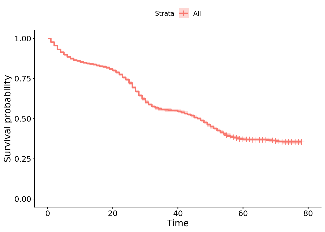
Median: 47 months 75: 24 months

# Use survminer::ggsurvplot() to plot the overall survival function.
survminer::ggsurvplot(fit = km_all)

Warning: Using `size` aesthetic for lines was deprecated in ggplot2 3.4.0.
ℹ Please use `linewidth` instead.
ℹ The deprecated feature was likely used in the ggpubr package.
  Please report the issue at <https://github.com/kassambara/ggpubr/issues>.

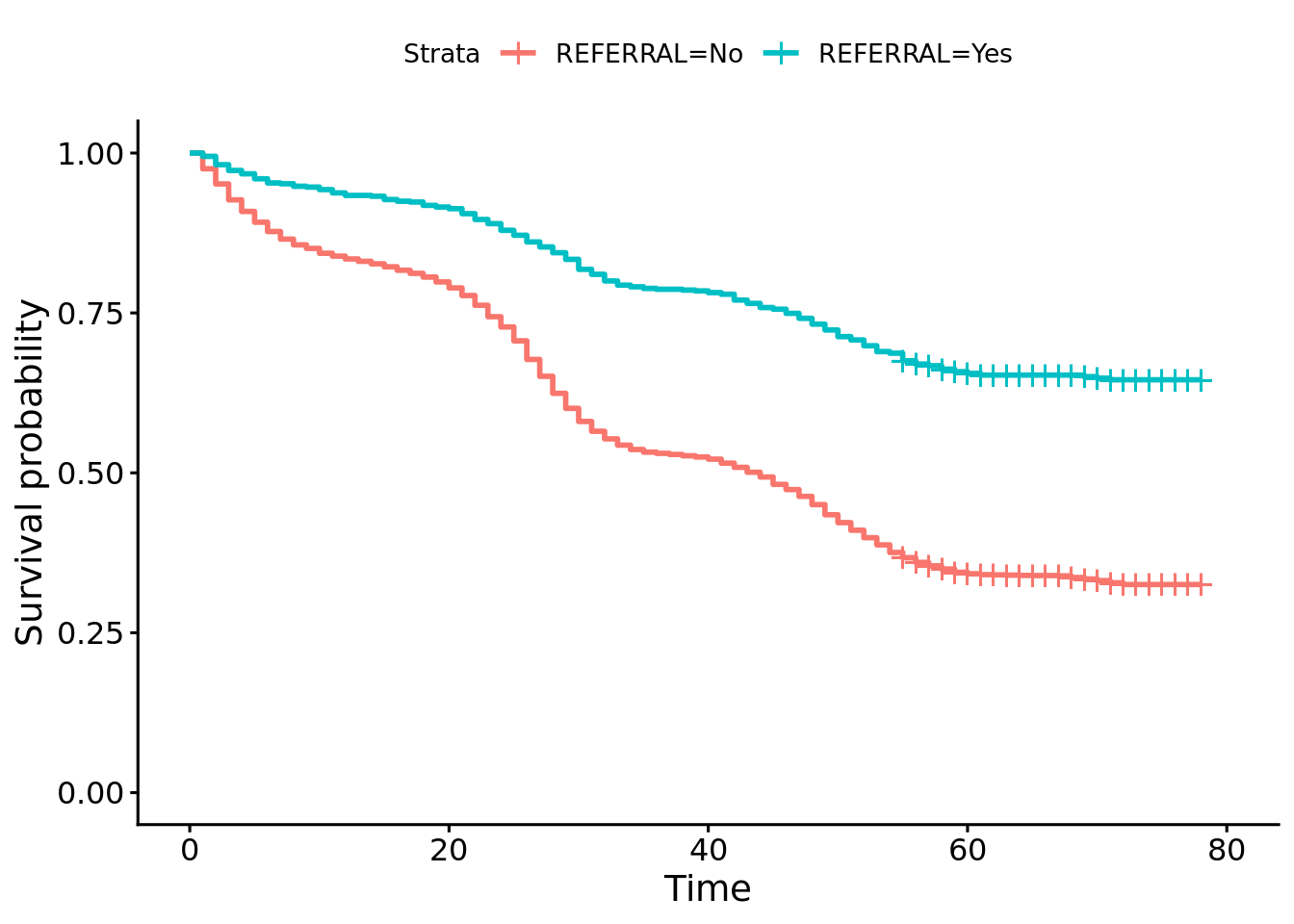
# Use survival::survfit() to estimate survival probabilities by the REFERRAL variable. 
# For the portion of the sample that was referred for the job (REFERRAL == "Yes"), how many months after hiring would you expect 50% of the sample to remain at the firm? What about for the portion of the sample that was not referred? 
# Why would the median survival time be missing? 

km_ref <- survival::survfit(surv_object ~ REFERRAL, data = surv_data)
summary(km_ref)

Call: survfit(formula = surv_object ~ REFERRAL, data = surv_data)

                REFERRAL=No 
 time n.risk n.event survival std.err lower 95% CI upper 95% CI
    1   7230     178    0.975 0.00182        0.972        0.979
    2   7052     171    0.952 0.00252        0.947        0.957
    3   6881     180    0.927 0.00306        0.921        0.933
    4   6701     131    0.909 0.00339        0.902        0.915
    5   6570     122    0.892 0.00365        0.885        0.899
    6   6448     105    0.877 0.00386        0.870        0.885
    7   6343      86    0.865 0.00401        0.858        0.873
    8   6257      65    0.856 0.00412        0.848        0.865
    9   6192      40    0.851 0.00419        0.843        0.859
   10   6152      55    0.843 0.00428        0.835        0.852
   11   6097      32    0.839 0.00432        0.830        0.847
   12   6065      32    0.834 0.00437        0.826        0.843
   13   6033      27    0.831 0.00441        0.822        0.839
   14   6006      28    0.827 0.00445        0.818        0.836
   15   5978      34    0.822 0.00450        0.813        0.831
   16   5944      39    0.817 0.00455        0.808        0.826
   17   5905      35    0.812 0.00460        0.803        0.821
   18   5870      42    0.806 0.00465        0.797        0.815
   19   5828      55    0.798 0.00472        0.789        0.808
   20   5773      67    0.789 0.00480        0.780        0.799
   21   5706      87    0.777 0.00489        0.768        0.787
   22   5619     110    0.762 0.00501        0.752        0.772
   23   5509     129    0.744 0.00513        0.734        0.754
   24   5380     116    0.728 0.00523        0.718        0.738
   25   5264     157    0.706 0.00536        0.696        0.717
   26   5107     210    0.677 0.00550        0.667        0.688
   27   4897     191    0.651 0.00561        0.640        0.662
   28   4706     192    0.624 0.00570        0.613        0.636
   29   4514     170    0.601 0.00576        0.590        0.612
   30   4344     148    0.580 0.00580        0.569        0.592
   31   4196     111    0.565 0.00583        0.554        0.577
   32   4085      86    0.553 0.00585        0.542        0.565
   33   3999      71    0.543 0.00586        0.532        0.555
   34   3928      49    0.537 0.00586        0.525        0.548
   35   3879      30    0.532 0.00587        0.521        0.544
   36   3849      14    0.530 0.00587        0.519        0.542
   37   3835      12    0.529 0.00587        0.517        0.540
   38   3823      15    0.527 0.00587        0.515        0.538
   39   3808      14    0.525 0.00587        0.513        0.536
   40   3794      24    0.521 0.00587        0.510        0.533
   41   3770      45    0.515 0.00588        0.504        0.527
   42   3725      48    0.509 0.00588        0.497        0.520
   43   3677      55    0.501 0.00588        0.490        0.513
   44   3622      54    0.493 0.00588        0.482        0.505
   45   3568      83    0.482 0.00588        0.471        0.494
   46   3485      59    0.474 0.00587        0.462        0.486
   47   3426      77    0.463 0.00586        0.452        0.475
   48   3349      93    0.450 0.00585        0.439        0.462
   49   3256     115    0.434 0.00583        0.423        0.446
   50   3141      89    0.422 0.00581        0.411        0.434
   51   3052      86    0.410 0.00578        0.399        0.422
   52   2966      84    0.399 0.00576        0.387        0.410
   53   2882      81    0.387 0.00573        0.376        0.399
   54   2801      86    0.376 0.00570        0.365        0.387
   55   2715      59    0.367 0.00567        0.356        0.379
   56   2638      53    0.360 0.00565        0.349        0.371
   57   2579      39    0.355 0.00563        0.344        0.366
   58   2534      35    0.350 0.00561        0.339        0.361
   59   2451      36    0.345 0.00559        0.334        0.356
   60   2376      16    0.342 0.00558        0.331        0.353
   61   2329       9    0.341 0.00558        0.330        0.352
   62   2256       2    0.341 0.00558        0.330        0.352
   63   2183       3    0.340 0.00558        0.329        0.351
   64   2058       3    0.340 0.00558        0.329        0.351
   65   1942       1    0.339 0.00558        0.329        0.351
   67   1227       2    0.339 0.00558        0.328        0.350
   68   1212       9    0.336 0.00560        0.326        0.348
   69   1189       8    0.334 0.00562        0.323        0.345
   70   1177       9    0.332 0.00564        0.321        0.343
   71   1143      12    0.328 0.00567        0.317        0.339
   72   1100       9    0.325 0.00570        0.314        0.337

                REFERRAL=Yes 
 time n.risk n.event survival std.err lower 95% CI upper 95% CI
    1    770       4    0.995 0.00259        0.990        1.000
    2    766      10    0.982 0.00481        0.972        0.991
    3    756       7    0.973 0.00587        0.961        0.984
    4    749       4    0.968 0.00639        0.955        0.980
    5    745       6    0.960 0.00708        0.946        0.974
    6    739       5    0.953 0.00761        0.938        0.968
    7    734       1    0.952 0.00771        0.937        0.967
    8    733       3    0.948 0.00800        0.933        0.964
    9    730       1    0.947 0.00809        0.931        0.963
   10    729       3    0.943 0.00836        0.927        0.959
   11    726       4    0.938 0.00871        0.921        0.955
   12    722       3    0.934 0.00896        0.916        0.951
   14    719       1    0.932 0.00904        0.915        0.950
   15    718       4    0.927 0.00936        0.909        0.946
   16    714       2    0.925 0.00951        0.906        0.944
   17    712       1    0.923 0.00959        0.905        0.942
   18    711       4    0.918 0.00988        0.899        0.938
   19    707       2    0.916 0.01002        0.896        0.935
   20    705       2    0.913 0.01016        0.893        0.933
   21    703       6    0.905 0.01056        0.885        0.926
   22    697       7    0.896 0.01100        0.875        0.918
   23    690       5    0.890 0.01129        0.868        0.912
   24    685       8    0.879 0.01174        0.857        0.903
   25    677       6    0.871 0.01206        0.848        0.895
   26    671       8    0.861 0.01247        0.837        0.886
   27    663       6    0.853 0.01275        0.829        0.879
   28    657       7    0.844 0.01307        0.819        0.870
   29    650       8    0.834 0.01342        0.808        0.860
   30    642      12    0.818 0.01390        0.791        0.846
   31    630       6    0.810 0.01413        0.783        0.839
   32    624       8    0.800 0.01441        0.772        0.829
   33    616       5    0.794 0.01459        0.765        0.823
   34    611       2    0.791 0.01465        0.763        0.820
   35    609       2    0.788 0.01472        0.760        0.818
   36    607       1    0.787 0.01475        0.759        0.816
   38    606       1    0.786 0.01479        0.757        0.815
   39    605       1    0.784 0.01482        0.756        0.814
   40    604       2    0.782 0.01488        0.753        0.812
   41    602       2    0.779 0.01495        0.750        0.809
   42    600       7    0.770 0.01516        0.741        0.800
   43    593       4    0.765 0.01528        0.736        0.795
   44    589       5    0.758 0.01543        0.729        0.789
   45    584       2    0.756 0.01548        0.726        0.787
   46    582       5    0.749 0.01562        0.719        0.781
   47    577       6    0.742 0.01578        0.711        0.773
   48    571       7    0.732 0.01595        0.702        0.764
   49    564       7    0.723 0.01612        0.692        0.756
   50    557       8    0.713 0.01630        0.682        0.746
   51    549       4    0.708 0.01639        0.676        0.741
   52    545       7    0.699 0.01653        0.667        0.732
   53    538       7    0.690 0.01667        0.658        0.723
   54    531       2    0.687 0.01671        0.655        0.721
   55    529       9    0.675 0.01687        0.643        0.709
   56    514       4    0.670 0.01695        0.638        0.704
   57    509       2    0.667 0.01698        0.635        0.702
   58    506       4    0.662 0.01705        0.630        0.696
   59    500       3    0.658 0.01710        0.626        0.693
   60    492       2    0.656 0.01714        0.623        0.690
   61    484       2    0.653 0.01717        0.620        0.687
   69    272       1    0.650 0.01728        0.617        0.685
   70    268       1    0.648 0.01738        0.615        0.683
   71    260       1    0.645 0.01749        0.612        0.681

Referral == “Yes” Median is undefined as more than 50% remain after end of study.

Referral == “No” Median: 44 months

# Use survminer::ggsurvplot() to plot the survival function by REFERRAL status. Are the two curves different? 
survminer::ggsurvplot(km_ref)

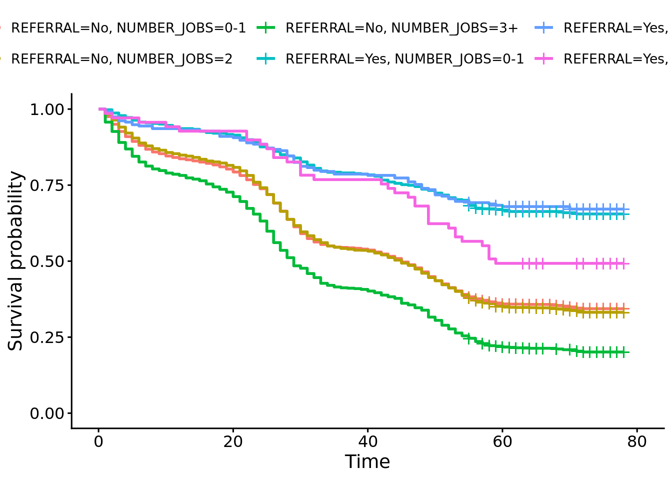
# Using the survfit function, estimate the survival probabilities for the interaction between REFERRAL and NUMBER_JOBS variables in 
# surv_data. Then plot the survival curve using ggsurvplot and provide an interpretation of the curves. Does their appear to be an
# interaction?
# 
# HINT: You don't need to create a new variable!  

km_ref_job <- survival::survfit(surv_object ~ REFERRAL + NUMBER_JOBS, data = surv_data)
survminer::ggsurvplot(km_ref_job)

Exercise 3 - Fit a cox proportional hazards model to your data.

# Estimate a cox proportional hazards model. Include all of the main effects and the interactions between INTPER_RATE and PROG_EXER_RATE as well as HIRE_REC and REFERRAL. 

# HINT: An interaction variable is created by multiplying Variable 1 with Variable 2 (Variable 1 * Variable 2).

mod_1 <- survival::coxph(
  surv_object ~ NUMBER_JOBS + PROG_EXER_RATE + 
    INTPER_RATE + PRIOR_EXP + HIRE_REC*REFERRAL + INTPER_RATE*PROG_EXER_RATE,
  data = surv_data
)

# View the coefficient estimates and standard errors of the model
summary(mod_1)

Call:
survival::coxph(formula = surv_object ~ NUMBER_JOBS + PROG_EXER_RATE + 
    INTPER_RATE + PRIOR_EXP + HIRE_REC * REFERRAL + INTPER_RATE * 
    PROG_EXER_RATE, data = surv_data)

  n= 8000, number of events= 5090 

                                    coef exp(coef) se(coef)      z Pr(>|z|)    
NUMBER_JOBS2                     0.01200   1.01207  0.03188  0.376   0.7067    
NUMBER_JOBS3+                    0.40501   1.49932  0.04401  9.204  < 2e-16 ***
PROG_EXER_RATEPass              -0.29343   0.74570  0.14419 -2.035   0.0418 *  
PROG_EXER_RATEPass+             -0.47220   0.62363  0.24214 -1.950   0.0512 .  
INTPER_RATE                     -0.10119   0.90376  0.01485 -6.816 9.38e-12 ***
PRIOR_EXPYes                    -0.01543   0.98469  0.03225 -0.478   0.6323    
HIRE_REC                        -0.08397   0.91946  0.01986 -4.227 2.36e-05 ***
REFERRALYes                     -0.90587   0.40419  0.19274 -4.700 2.60e-06 ***
HIRE_REC:REFERRALYes            -0.02592   0.97441  0.08550 -0.303   0.7618    
PROG_EXER_RATEPass:INTPER_RATE   0.00691   1.00693  0.01700  0.406   0.6844    
PROG_EXER_RATEPass+:INTPER_RATE  0.01875   1.01893  0.02841  0.660   0.5093    
---
Signif. codes:  0 '***' 0.001 '**' 0.01 '*' 0.05 '.' 0.1 ' ' 1

                                exp(coef) exp(-coef) lower .95 upper .95
NUMBER_JOBS2                       1.0121     0.9881    0.9508    1.0773
NUMBER_JOBS3+                      1.4993     0.6670    1.3754    1.6344
PROG_EXER_RATEPass                 0.7457     1.3410    0.5621    0.9892
PROG_EXER_RATEPass+                0.6236     1.6035    0.3880    1.0024
INTPER_RATE                        0.9038     1.1065    0.8778    0.9304
PRIOR_EXPYes                       0.9847     1.0156    0.9244    1.0489
HIRE_REC                           0.9195     1.0876    0.8843    0.9560
REFERRALYes                        0.4042     2.4741    0.2770    0.5897
HIRE_REC:REFERRALYes               0.9744     1.0263    0.8241    1.1522
PROG_EXER_RATEPass:INTPER_RATE     1.0069     0.9931    0.9739    1.0411
PROG_EXER_RATEPass+:INTPER_RATE    1.0189     0.9814    0.9637    1.0773

Concordance= 0.59  (se = 0.004 )
Likelihood ratio test= 621.4  on 11 df,   p=<2e-16
Wald test            = 573.6  on 11 df,   p=<2e-16
Score (logrank) test = 596.4  on 11 df,   p=<2e-16

# Estimate a cox proportional hazards model that only includes the main effects (no interactions).
mod_2 <- survival::coxph(
  surv_object ~ NUMBER_JOBS + PROG_EXER_RATE + 
    INTPER_RATE + PRIOR_EXP + HIRE_REC + REFERRAL,
  data = surv_data
)

# View the coefficient estimates and standard errors for the main effects model. 
summary(mod_2)

Call:
survival::coxph(formula = surv_object ~ NUMBER_JOBS + PROG_EXER_RATE + 
    INTPER_RATE + PRIOR_EXP + HIRE_REC + REFERRAL, data = surv_data)

  n= 8000, number of events= 5090 

                         coef exp(coef)  se(coef)       z Pr(>|z|)    
NUMBER_JOBS2         0.011914  1.011985  0.031884   0.374    0.709    
NUMBER_JOBS3+        0.404358  1.498340  0.043982   9.194  < 2e-16 ***
PROG_EXER_RATEPass  -0.236436  0.789437  0.034121  -6.929 4.23e-12 ***
PROG_EXER_RATEPass+ -0.316998  0.728333  0.055603  -5.701 1.19e-08 ***
INTPER_RATE         -0.094790  0.909564  0.006966 -13.607  < 2e-16 ***
PRIOR_EXPYes        -0.015768  0.984356  0.032248  -0.489    0.625    
HIRE_REC            -0.085417  0.918129  0.019324  -4.420 9.86e-06 ***
REFERRALYes         -0.962249  0.382033  0.062635 -15.363  < 2e-16 ***
---
Signif. codes:  0 '***' 0.001 '**' 0.01 '*' 0.05 '.' 0.1 ' ' 1

                    exp(coef) exp(-coef) lower .95 upper .95
NUMBER_JOBS2           1.0120     0.9882    0.9507    1.0772
NUMBER_JOBS3+          1.4983     0.6674    1.3746    1.6332
PROG_EXER_RATEPass     0.7894     1.2667    0.7384    0.8440
PROG_EXER_RATEPass+    0.7283     1.3730    0.6531    0.8122
INTPER_RATE            0.9096     1.0994    0.8972    0.9221
PRIOR_EXPYes           0.9844     1.0159    0.9241    1.0486
HIRE_REC               0.9181     1.0892    0.8840    0.9536
REFERRALYes            0.3820     2.6176    0.3379    0.4319

Concordance= 0.59  (se = 0.004 )
Likelihood ratio test= 620.9  on 8 df,   p=<2e-16
Wald test            = 572.2  on 8 df,   p=<2e-16
Score (logrank) test = 590.3  on 8 df,   p=<2e-16

# Compare the model you fit above to a model that only includes the main effects (no interactions). Use the anova() function to determine if the model with interactions fits your data significantly better than the model with main effects only. If you are unsure of how to use the anova() function, then view the help documentation on it ?anova.coxph or exercise solutions.  
anova(mod_1, mod_2)

Analysis of Deviance Table
 Cox model: response is  surv_object
 Model 1: ~ NUMBER_JOBS + PROG_EXER_RATE + INTPER_RATE + PRIOR_EXP + HIRE_REC * REFERRAL + INTPER_RATE * PROG_EXER_RATE
 Model 2: ~ NUMBER_JOBS + PROG_EXER_RATE + INTPER_RATE + PRIOR_EXP + HIRE_REC + REFERRAL
  loglik Chisq Df P(>|Chi|)
1 -43245                   
2 -43245 0.551  3    0.9076

# Based on the model comparison above, decide if you should choose the more complicated interaction model or the less complicated main effects model. Using the model you decided on, test the proportional hazard assumption and determine if any variables violate it. If they do decide if you should drop them from the model.
survival::cox.zph(mod_2)

               chisq df     p
NUMBER_JOBS    2.461  2 0.292
PROG_EXER_RATE 1.294  2 0.523
INTPER_RATE    0.129  1 0.720
PRIOR_EXP      3.790  1 0.052
HIRE_REC       1.542  1 0.214
REFERRAL       0.174  1 0.677
GLOBAL         9.414  8 0.309

mod <- survival::coxph(
  surv_object ~ REFERRAL + NUMBER_JOBS + PROG_EXER_RATE + 
    INTPER_RATE + HIRE_REC,
  data = surv_data
)

Prior experience is close to violating the assumption and is unrelated to attrition, so we can safely drop it from the model ## Exercise 4 - Interpreting the proportional hazards results.

# Using the final model you decided on during last exercise, provide an interpretation of each of the predictors you kept in the model. 
summary(mod)

Call:
survival::coxph(formula = surv_object ~ REFERRAL + NUMBER_JOBS + 
    PROG_EXER_RATE + INTPER_RATE + HIRE_REC, data = surv_data)

  n= 8000, number of events= 5090 

                         coef exp(coef)  se(coef)       z Pr(>|z|)    
REFERRALYes         -0.962134  0.382077  0.062635 -15.361  < 2e-16 ***
NUMBER_JOBS2         0.012290  1.012366  0.031874   0.386      0.7    
NUMBER_JOBS3+        0.404310  1.498268  0.043982   9.193  < 2e-16 ***
PROG_EXER_RATEPass  -0.236269  0.789568  0.034119  -6.925 4.37e-12 ***
PROG_EXER_RATEPass+ -0.316808  0.728470  0.055602  -5.698 1.21e-08 ***
INTPER_RATE         -0.094830  0.909528  0.006966 -13.613  < 2e-16 ***
HIRE_REC            -0.085499  0.918054  0.019324  -4.425 9.66e-06 ***
---
Signif. codes:  0 '***' 0.001 '**' 0.01 '*' 0.05 '.' 0.1 ' ' 1

                    exp(coef) exp(-coef) lower .95 upper .95
REFERRALYes            0.3821     2.6173    0.3379    0.4320
NUMBER_JOBS2           1.0124     0.9878    0.9511    1.0776
NUMBER_JOBS3+          1.4983     0.6674    1.3745    1.6332
PROG_EXER_RATEPass     0.7896     1.2665    0.7385    0.8442
PROG_EXER_RATEPass+    0.7285     1.3727    0.6533    0.8123
INTPER_RATE            0.9095     1.0995    0.8972    0.9220
HIRE_REC               0.9181     1.0893    0.8839    0.9535

Concordance= 0.59  (se = 0.004 )
Likelihood ratio test= 620.6  on 7 df,   p=<2e-16
Wald test            = 571.8  on 7 df,   p=<2e-16
Score (logrank) test = 590  on 7 df,   p=<2e-16

Referral reduces hazard by a factor of .38 (~62%). No difference between 0-1 and 2 jobs prior to hiring. Having 3+ jobs in the year before hire increases hazard by a factor of 1.50 (50%). Compared to a “Concerns” rating on the programming exercise, Pass and Pass+ both reduce hazard by factors of .79 (21%) and .73 (27%), respectively. Every unit increase in interpersonal skills reduces the hazard by a factor of .91 (9%). Every additional increase in hiring rec reduces hazard by a factor of .92 (8%).

# Use the function confint() to calculate the 95% confidence intervals for each coefficient.
# Transform the confidence intervals so that they can be interpreted as confidence intervals for exp(coef).
confint(mod)

                         2.5 %      97.5 %
REFERRALYes         -1.0848963 -0.83937218
NUMBER_JOBS2        -0.0501824  0.07476316
NUMBER_JOBS3+        0.3181076  0.49051261
PROG_EXER_RATEPass  -0.3031419 -0.16939606
PROG_EXER_RATEPass+ -0.4257857 -0.20783126
INTPER_RATE         -0.1084834 -0.08117663
HIRE_REC            -0.1233720 -0.04762507

exp(confint(mod))

                        2.5 %    97.5 %
REFERRALYes         0.3379368 0.4319816
NUMBER_JOBS2        0.9510559 1.0776289
NUMBER_JOBS3+       1.3745241 1.6331532
PROG_EXER_RATEPass  0.7384943 0.8441745
PROG_EXER_RATEPass+ 0.6532563 0.8123441
INTPER_RATE         0.8971938 0.9220308
HIRE_REC            0.8839348 0.9534912

Exercise 5 - Creating predicted survival curves from your proportional hazards model.

# Create a new data frame that contains a column for each of the variables you included in your Cox regression model. Pick of variable you are interested in and provide different values for that variable (the values need to occur in the original data frame) while holding the other variables constant (e.g. NUMBER_JOBS == "0-1" for all rows in the new data frame).
new_data <- data.frame(REFERRAL = c("No", "Yes"), 
                       NUMBER_JOBS = c("3+", "3+"), 
                       PROG_EXER_RATE = c("Concerns", "Concerns"), 
                       INTPER_RATE = c(1, 1), 
                       PRIOR_EXP = c("No", "No"), 
                       HIRE_REC = c(0, 0))

# With your new data frame and your estimated Cox regression model, use the function: survival::survfit() to create predicted survival probabilities from your model and new data frame. 
# Using summary(), explore these new probabilities. 
predicted_surv_prob <- survival::survfit(mod, newdata = new_data)
summary(predicted_surv_prob)

Call: survfit(formula = mod, newdata = new_data)

 time n.risk n.event survival1 survival2
    1   8000     182   0.90443     0.962
    2   7818     181   0.81626     0.925
    3   7637     187   0.73205     0.888
    4   7450     135   0.67541     0.861
    5   7315     128   0.62480     0.836
    6   7187     110   0.58362     0.814
    7   7077      87   0.55252     0.797
    8   6990      68   0.52909     0.784
    9   6922      41   0.51533     0.776
   10   6881      58   0.49631     0.765
   11   6823      36   0.48477     0.758
   12   6787      35   0.47374     0.752
   13   6752      27   0.46536     0.747
   14   6725      29   0.45648     0.741
   15   6696      38   0.44504     0.734
   16   6658      41   0.43293     0.726
   17   6617      36   0.42250     0.720
   18   6581      46   0.40945     0.711
   19   6535      57   0.39370     0.700
   20   6478      69   0.37524     0.688
   21   6409      93   0.35140     0.671
   22   6316     117   0.32306     0.649
   23   6199     134   0.29276     0.625
   24   6065     124   0.26667     0.604
   25   5941     163   0.23509     0.575
   26   5778     218   0.19733     0.538
   27   5560     197   0.16728     0.505
   28   5363     199   0.14057     0.473
   29   5164     178   0.11955     0.444
   30   4986     160   0.10278     0.419
   31   4826     117   0.09171     0.401
   32   4709      94   0.08349     0.387
   33   4615      76   0.07728     0.376
   34   4539      51   0.07330     0.368
   35   4488      32   0.07089     0.364
   36   4456      15   0.06978     0.362
   37   4441      12   0.06890     0.360
   38   4429      16   0.06774     0.358
   39   4413      15   0.06667     0.355
   40   4398      26   0.06484     0.352
   41   4372      47   0.06163     0.345
   42   4325      55   0.05804     0.337
   43   4270      59   0.05436     0.329
   44   4211      59   0.05087     0.320
   45   4152      85   0.04613     0.309
   46   4067      64   0.04280     0.300
   47   4003      83   0.03875     0.289
   48   3920     100   0.03428     0.276
   49   3820     122   0.02936     0.260
   50   3698      97   0.02586     0.247
   51   3601      90   0.02290     0.236
   52   3511      91   0.02017     0.225
   53   3420      88   0.01778     0.214
   54   3332      88   0.01561     0.204
   55   3244      68   0.01408     0.196
   56   3152      57   0.01288     0.190
   57   3088      41   0.01207     0.185
   58   3040      39   0.01133     0.181
   59   2951      39   0.01061     0.176
   60   2868      18   0.01029     0.174
   61   2813      11   0.01009     0.173
   62   2726       2   0.01006     0.172
   63   2645       3   0.01000     0.172
   64   2496       3   0.00994     0.172
   65   2353       1   0.00992     0.172
   67   1502       2   0.00986     0.171
   68   1485       9   0.00957     0.169
   69   1461       9   0.00928     0.167
   70   1445      10   0.00897     0.165
   71   1403      13   0.00856     0.162
   72   1348       9   0.00829     0.160

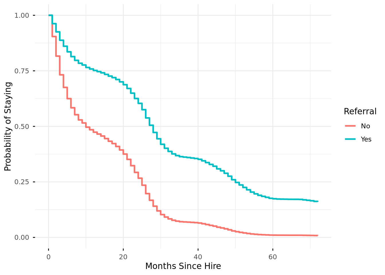
# With your new data frame and your estimated Cox regression model, use the function: survminer::ggadjustedcurves() to plot your predicted survival functions. If you are familiar with ggplot2, then try to customize the plot output. 
survminer::ggadjustedcurves(mod, 
                            data = new_data, variable = "REFERRAL", 
                            ylab = "Probability of Staying",
                            xlab = "Months Since Hire",
                            ggtheme = ggplot2::theme_minimal()) +
  ggplot2::labs(color = "Referral")

Using the results of your final Cox regression model and your predicted survival functions to write a high-level business summary of what predictor or predictors you believe to be the most important to focus on to reduce attrition.